2.3 Matrices and matrix calculations

2.3.1 Defining and using matrices

Matrices can be defined using square brackets. Example 2.2 shows how this is accomplished. It also shows how to define matrices using other matrices as blocks and how to perform basic arithmetic operations on matrices.

■ Example 2.2
▼ Input	▼ Output
// A is a 2x3 matrix  A = [1, 2, 3;       4, 5, 6];  print(A);    // White space is irrelevant. All  // that matters is that columns are  // separated by "," and rows by ";".  B = [1,2,3; 4,5,6];  print(B);    // B is equal to A  print(A-B);    // Arithmetic operations on matrices  C = 3*A - 2*(B+A);  print(C);    // Take the transpose of C  D = C′;  print(D);    // Create E by defining its blocks:  // 1 -> a 3x1 vector  // 2 -> a 3x2 matrix  E = [ [1;2;3], 2*D ];  print(E);	A =    1  2  3    4  5  6      B =    1  2  3    4  5  6      A-B =    0  0  0    0  0  0      C =    -1  -2  -3    -4  -5  -6      D =    -1  -4    -2  -5    -3  -6      E =      1   -2   -8      2   -4  -10      3   -6  -12

2.3.2 Indexing matrices and the range operator

The entries of matrices can be accessed using parentheses after the matrix id value. For example, if A is a matrix currently in memory, the statement:

will take the element of A located in the 3^rd row, 4^th column and store it in an item with id value b.

When you want to access consecutive entries in a matrix you have to use the range operator, “:". When the range operator is preceded and followed by positive integers, i and j, respectively, with i $<$ j, it is taken to mean “from i to j". For example, the statement:

will take the entries of A located in rows 2 to 3, column 4 and store them in a $2\times 1$ matrix C.

When the range operator is not preceded and not followed by integers, it is taken to mean “all items in the respective dimension". For example, the statement:

will take the entire 4^th column of A and store it in a matrix (column vector) D.

Finally, when a single range operator is used to index the elements of a vector or matrix, A, then all entries of A are requested. That is, all three statements:

are equivalent when A is a matrix, and they create a copy of A into a matrix with id value D.

Example 2.3 puts all these together, while Example 2.4 shows how indexing is performed and how the range operator can be used in the left-hand side of assignment statements to alter a block of a matrix already in memory. It also shows how to copy the entries of a matrix A into another matrix B, respecting the dimensions of the left-hand-side matrix.

■ Example 2.3
▼ Input	▼ Output
// Define A as a 4x4 matrix  A = [ 1, 2, 3, 4;       -1,-2,-3,-4;        8, 7, 6, 5;       -4,-5,-6,-8      ];    // b is the entry of A in row 3,  // column 4  b = A(3,4);  print(b);    // Print the elements in rows 2 to 3,  // column 4  print(A(2:3,4));    // Print the 4th column of A  print(A(:,4));    // Print the 1st row of A  print(A(1,:));	b =    5      A(2:3,4) =    -4    5      A(:,4) =    4    -4    5    -8      A(1,:) =    1  2  3  4

■ Example 2.4
▼ Input	▼ Output
/* Define A as a 3x2 matrix of random  draws from an exponential distribution  with rate 2.5 and print it */  A = exprnd(2.5,3,2);  print(A);    // Make the entry in row 2, column 1  // of A equal to one and print A  A(2,1) = 1;  print(A);    // Make the first row of A equal to a  // vector of zeros  A(1,:) = zeros(1, cols(A));  print(A);    // Define B as a 3x2 matrix of zeros  // and assign the entries of A to it  B = zeros(2,3);  B(:) = A;  print(A);  print(B);    /* A and B have different dimensions  but the same number of entries. The  entries of A are stored in B in a  column-major fashion */	A =     0.20604   1.10341    0.170939  0.142362    0.535967  0.360443      A =     0.20604   1.10341           1  0.142362    0.535967  0.360443      A =           0         0           1  0.142362    0.535967  0.360443      A =           0         0           1  0.142362    0.535967  0.360443      B =           0  0.535967  0.142362           1         0  0.360443

2.3.3 Element-wise operators

Matrix addition and subtraction work, as expected, in an element-wise fashion: if $\mathbf{A}$ and $\mathbf{B}$ are two $M\times N$ matrices and $\mathbf{C}=\mathbf{A}+\mathbf{B}$, then $\mathbf{C}$ is defined such that $c_{ij}=a_{ij}+b_{ij}$, $\forall i=1,\dots M,j=1,\dots N$. Matrix-matrix multiplication, again as expected, works in a non-element-wise fashion: if $\mathbf{A}$ is an $M\times K$ matrix, $\mathbf{B}$ is a $K\times N$ matrix and $\mathbf{C}=\mathbf{A}\cdot \mathbf{B}$, then $\mathbf{C}$ is an $M\times N$ matrix such that:

$$c_{ij}=\sum _{k=1}^K{a}_{ik}\cdot b_{kj}\forall i=1,\dots M,j=1,\dots N$$

However, very frequently in practice, one needs to do element-wise multiplication, division or exponentiation of matrices. As it is common in other matrix languages, BayES defines the following element-wise operators:

• “.*" for element-wise multiplication
• “./" for element-wise division
• “.^" for element-wise exponentiation

Example 2.5 shows how these operators can be used.

■ Example 2.5
▼ Input	▼ Output
// Define matrices  A = [ 1, 2;        3, 4];  B = [ 5, 4;        2, 1];    // Element-wise multiplication  print(A.*B);    // Element-wise division  print(A./B);    // Element-wise exponentiation  print(A.^B);	A.*B =    5  8    6  4      A./B =    0.2  0.5    1.5    4      A.^B =     1  16     9   4

2.3.4 Operator precedence

Arithmetic operations contained in an expression are evaluated in the following order:

Operators with equal precedence are evaluated from left to right.

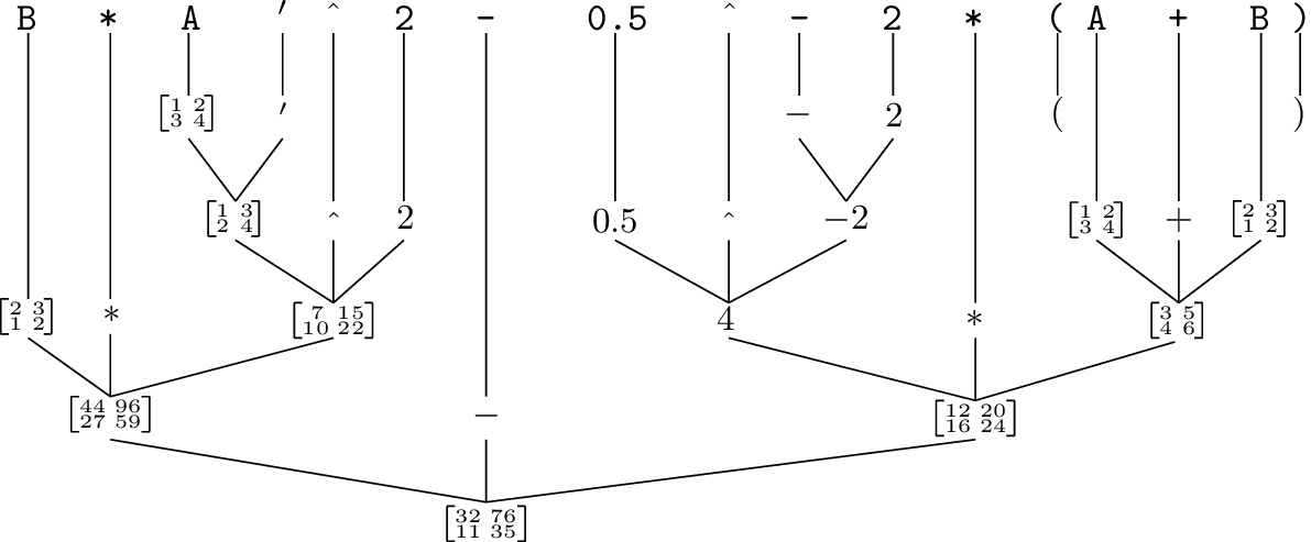
As an example, consider the expression:

where A and B are $2\times 2$ matrices:

The expression above is evaluated in the following way:

2.3.5 Functions operating on matrices

BayES provides an array of functions that take matrices as arguments and return matrices. These include:

• special matrix functions like inv(), trace(), diag(), etc.
• functions that provide generalizations of scalar functions like log(), exp(), sqrt(), etc. to matrices and work in an element-wise fashion
• summing, rounding and descriptive-statistics functions like sum(), floor(), mean(), etc.
• decompositions of matrices like chol() and eig()

Detailed descriptions of these functions are given in Appendix B.

Share this content:

© 2016–20 Grigorios Emvalomatis