2.11 Plotting

BayES provides functions for producing elementary graphics. The following types of plots are supported:

Section B.16 provides extensive documentation on the plotting functions. The remainder of this section gives a general overview of how plots are handled in BayES and presents some simple examples.

When a plotting function is called in BayES in its simple form, a new figure window is created and the corresponding plot is drawn within this window. Figure windows are named consecutively as "Figure 1", "Figure 2", etc., and these names can be used to interact with them, for example to close them programmatically or save their plots in any of the supported graphics formats. For example, the statement:

will close the figure window with "Figure 2" appearing on its title bar and release the memory occupied by this figure. To prevent extreme use of memory resources for presenting plots, BayES restricts the maximum number of figure windows that are open simultaneously to 20. This number can be changed using the maxfigures() function.

Once a figure window is closed, its name will be reused. For example, if there are currently two figure windows open with titles "Figure 1" and "Figure 3" (the user closed the figure window with title "Figure 2"), the next time a plotting function is used, the title of the new figure window will be "Figure 2". The statement:

closes all currently open figure windows and releases resources.

The titles of figure windows can also be used to export the associated plots to the following graphics formats:

This is achieved using the export() function, by passing the name of the figure window that contains the plot to be exported as the first argument of the export() function. Section B.4 provides extensive documentation on the export() function.

The five basic plotting functions mentioned above differ in the number of numerical arguments they take, but all of them have the following optional arguments:

• "title"
• "xlabel"
• "ylabel"
• "grid"
• "colors"

These arguments, if provided, must be given after the numerical arguments of the respective plotting function, separated by commas.⁸ The values of the first four options should be strings and of the "colors" option a matrix. The three first options, as presented above, specify the title of the plot and the labels on the ‘x’ and ‘y’ axes, respectively. The values of the "grid" option must equal to either "on" or "off", with the first value requesting that a grid is plotted on the graph. The last option specifies the colors to be used in the graph and its value must a matrix with three columns and, possibly, multiple rows. The values in each row represent a color in RGB (red-green-blue) format and should be between zero and one. The first row specifies the background color of the graph⁹ and the second the color of the axes and text labels. The remaining rows specify the colors to be used when plotting the data.

BayES provides support for figure windows which can contain multiple plots. A call to the multiplot() function will initialize a figure window which can store multiple plots. Subsequent calls to the five basic plotting functions, accompanied by calls to the subplot() function, can be used to populate the spaces of this window with actual plots. See section B.16 for more details.

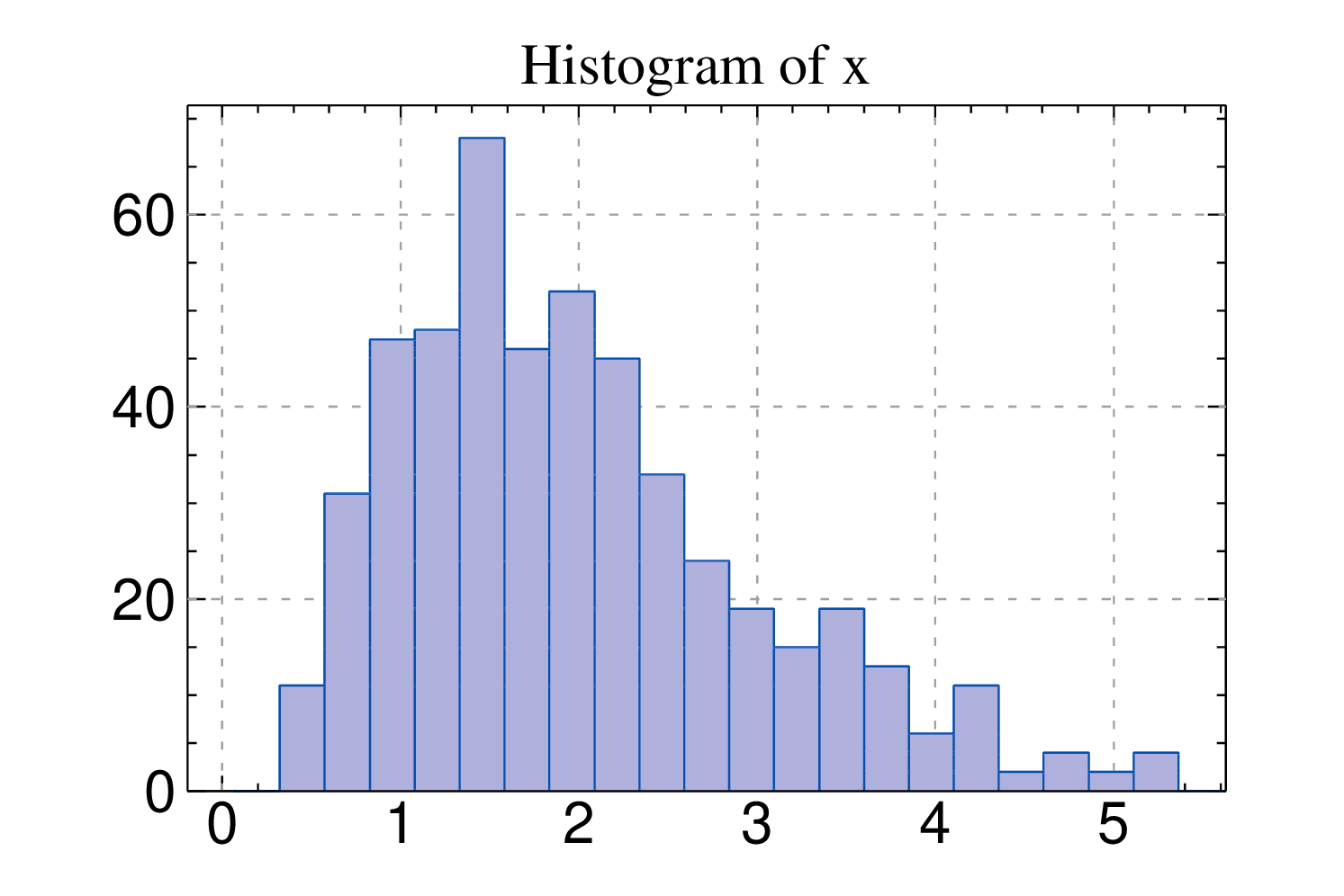
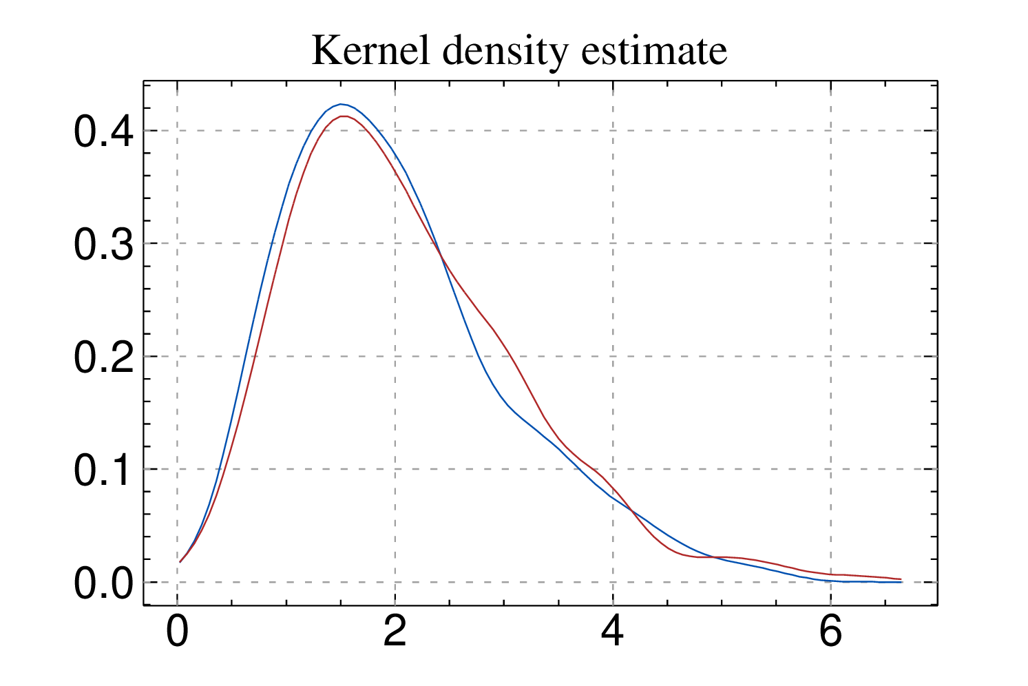
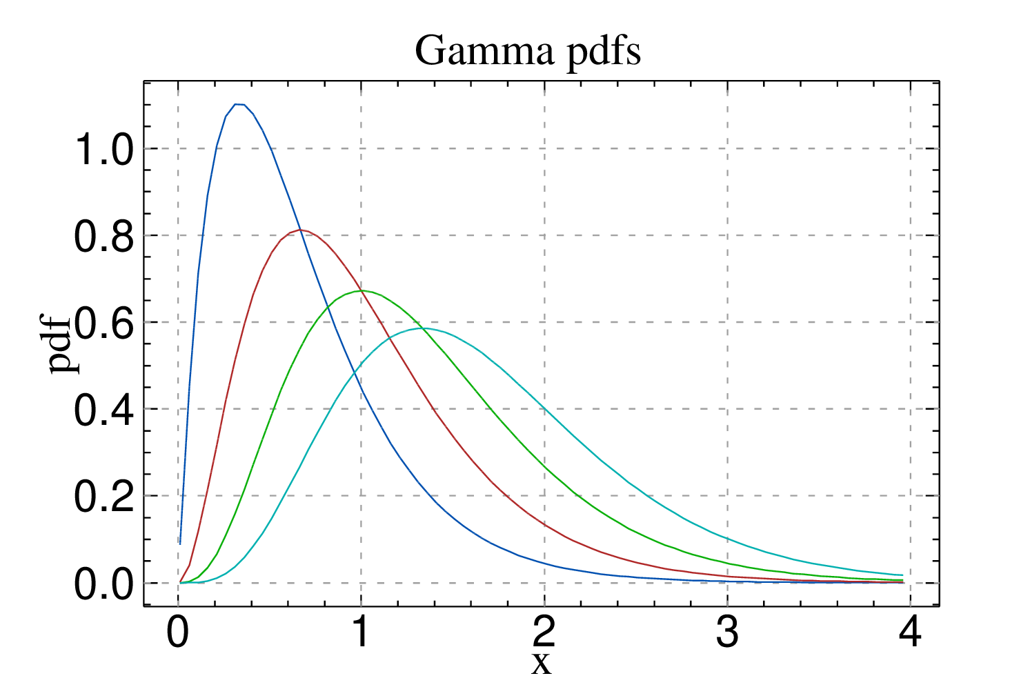
Example 2.11 demonstrates how to plot a histogram of a set of values contained in a vector, while example 2.12 shows how to overlay kernel density estimates of the values contained in two vectors. Finally, 2.13 demonstrates how to plot a set of functions. Sample "4$-$Plotting data.bsf", located at "$BayESHOME/Samples/1$-$GettingStarted" contains some more complete examples of using the plotting functions.

■ Example 2.11
▼ Input	▼ Output
// Set the seed for the random-number  // generator and draw 500 numbers from  // a Gamma(4,2) distribution  seed(42);  x = gamrnd(4,2,500,1);    // Plot a histogram of the values in x  hist(x, 20,      "title"="Histogram of x",      "grid"="on" );    // Export the graph as eps  export( "Figure 1", "./Hist.eps",      "width"=420, "height"=280 );

■ Example 2.12
▼ Input	▼ Output
// Draw two sets of 500 numbers from  // a Gamma(4,2) distribution  seed(42);  x = gamrnd(4,2,500,1);  y = gamrnd(4,2,500,1);    // Overlay the kernel density estima-  // tes for the values in x and y  kden( [ x, y ],      "title"="Kernel density estimate",      "grid"="on" );    // Export the graph as eps  export( "Figure 1", "./Kden.eps",      "width"=420, "height"=280 );

■ Example 2.13
▼ Input	▼ Output
// Define x-axis values  x = range(0.01, 4, 0.05);    // Plot the Gamma pdf with varying  // shape parameter  y1 = gampdf(x, 2, 3);  y2 = gampdf(x, 3, 3);  y3 = gampdf(x, 4, 3);  y4 = gampdf(x, 5, 3);  myPlot = plot( [ y1, y2, y3, y4 ], x,      "title" = "Gamma pdfs",      "xlabel" = "x", "ylabel" = "pdf",      "grid"="on" );    // Export the graph as eps  export( myPlot, "./Gampdf.eps",      "width"=420, "height"=280 );

Share this content:

© 2016–20 Grigorios Emvalomatis